Excel Waterfall Chart Template With Negative Values. Add new values by inserting rows and copying formulas down no macros using the chart in another workbook Download this table in excel (.xls) format, and complete it with your specific information.
6 Excel Waterfall Chart Template with Negative Values Excel Templates Excel Templates from www.exceltemplate123.us
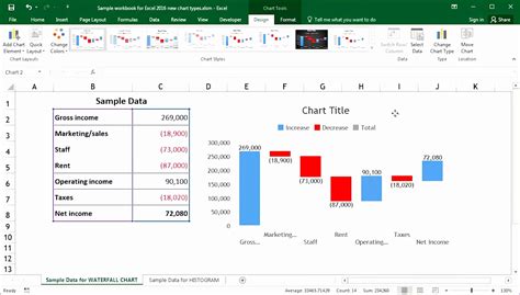
Your chart will automatically be created based on the values in our template. Summary of features allows negative values includes dashed horizontal connecting lines Sometimes they’re also called bridge charts because of the connector lines which may be included to link each data point.
Waterfall Charts Basically List Down All The Positive And Negative Values For A Certain.
Download waterfall chart template a waterfall chart (also called a bridge chart, flying bricks chart, cascade chart, or mario chart) is a graph that visually breaks down the cumulative effect that a series of sequential positive or negative values have contributed to the final outcome. A waterfall chart or bridge chart can be a great way to visualize adjustments made to an initial value, such as the breakdown of expenses in an income statement leading to a final net income value. It’s one of the most visually descriptive charts supported in excel.
Also Scroll Down For The Workbook.
Insert a waterfall chart in excel. These kinds of charts are also known as bridge charts (showing a connection between following bar graphs) or mario charts. Click either of the before or after series lines, click the green plus button on the top right corner of the waterfall chart and check the box for up/down bars.
It Uses Simple But Unusual Techniques To Quickly And Easily Get A Waterfall Chart That Also Works With Negative Cumulative Values.
For the complete course with different variations of the waterfall chart click here: Now select the entire data range go to insert >charts >column >under column chart > select stacked column as shown in the below screenshot. Your chart should now look like this:
You Will Get The Chart As Below.
Create waterfall chart in excel 2016 and later versions; A waterfall chart represents data visualization of cumulative effect on initial value from sequential introduction of intermediate negative or positive values. Complex with previous versions of excel (2013, 2010, etc.), the waterfall graph is created in a few clicks in the 2016 and 2019 versions.
To Be Able To Use These Models Correctly, You Must First Activate The Macros At Startup.
A waterfall chart template is, simply put, another way of data visualization, it is also called the bridge. The columns are color coded so you can quickly tell positive from negative numbers. At this point, all the hard work is done.